Last Update: June 20, 2022
ARIMA Models Identification: Correlograms are used to identify ARIMA models autoregressive and moving average orders.
As example, we can delimit univariate time series into training range
for model fitting and testing range
for model forecasting.
Then, we can do training range univariate time series model autoregressive
and moving average
orders identification by estimating sample autocorrelation and partial autocorrelation functions correlograms. Notice that we need to evaluate whether level or
order differentiated training range univariate time series is needed for ARIMA model integration
order.
Next, we estimate training range univariate time series sample autocorrelation function correlogram with formula . Training range univariate time series estimated lag
sample autocorrelation function
is the estimated sample covariance between univariate time series
and its lag
univariate time series
divided by univariate time series estimated sample variance
. Training range autocorrelation function is the linear dependence between current
and lagged
univariate time series data.
After that, we estimate training range sample autocorrelation function correlogram confidence intervals with formula . Training range sample autocorrelation function confidence intervals
are the inverse of the standard normal cumulative distribution
with probability equal to one minus statistical significance level
divided by two and this result multiplied by the square root of one plus two times the sum of sample autocorrelation function square values
divided by number of observations
. Notice that we need to evaluate whether Bartlett formula is needed for sample autocorrelation function correlogram confidence intervals estimation.
Later, we estimate training range univariate time series sample partial autocorrelation function correlogram with formula . Training range univariate time series lag
sample partial autocorrelation function
can be estimated through lag
linear regression estimated coefficient
with formula
. Training range partial autocorrelation function is the linear dependence between current
and lagged
univariate time series data after removing any linear dependence on
. Notice that we can also estimate sample partial autocorrelation function using Yule-Walker, Levison-Durbin or adjusted linear regression methods.
Then, we estimate training range sample partial autocorrelation function correlogram confidence intervals with formula . Training range sample partial autocorrelation function confidence intervals
are the inverse of the standard normal cumulative distribution
with probability equal to one minus statistical significance level
divided by two and this result multiplied by one divided by the square root of number of observations
.
Next, we can do training range univariate time series model autoregressive
and moving average
orders identification.
- If sample autocorrelation function correlogram
tails of gradually and sample partial autocorrelation function correlogram
drops after
statistically significant lags then we can observe the potential need of an autoregressive model
of order
- Alternatively, if sample autocorrelation function correlogram
statistically significant lags and sample partial autocorrelation function correlogram
of order
- Otherwise, if sample autocorrelation function correlogram
of orders
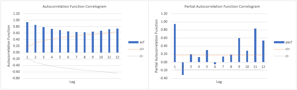
Below, we find example of training range univariate time series model autoregressive
and moving average
orders identification correlograms using airline passengers data [1]. Training range as first ten years and testing range as last two years of data. Correlograms confidence intervals with
statistical significance level. Notice that correlograms confidence intervals statistical significance level was only included as an educational example which can be modified according to your needs.
References
[1] Data Description: Monthly international airline passenger numbers in thousands from 1949 to 1960.
Original Source: Box, G. E. P., Jenkins, G. M. and Reinsel, G. C. (1976). “Time Series Analysis, Forecasting and Control”. Third Edition. Holden-Day. Series G.
Source: datasets R Package AirPassengers Object. R Core Team (2021). “R: A language and environment for statistical computing”. R Foundation for Statistical Computing, Vienna, Austria.