Last Update: March 24, 2022
Exogeneity is when linear regression independent variables are not correlated with error term. This can be tested through Wu-Hausman test [1] which evaluates whether linear regression independent variables are not correlated with error term (exogenous). If linear regression independent variables are correlated with error term (endogenous), then instrumental variables and two stage least squares estimation are used.
Instrumental variables have the following requirements. They are not included within original linear regression, they are assumed correlated with endogenous independent variable and they are assumed not correlated with second stage least squares linear regression error term. Last requirement can be tested through Sargan test [2] which evaluates whether instrumental variables are not correlated with second stage least squares linear regression error term (valid instruments). If instrumental variables are correlated with second stage least squares linear regression error term, then they are instruments not valid.
As example, we can fit a three-variable original multiple linear regression with formula . Original linear regression fitted values
are the estimated
values,
is the endogenous independent variable (assumed correlated with original linear regression error term),
is the exogenous independent variable (assumed not correlated with original linear regression error term). Then, we can fit first stage least squares multiple linear regression with formula
. First stage least squares linear regression fitted values
are the estimated
values,
and
are the instrumental variables. Next, we can fit second stage least squares multiple linear regression with formula
. Second stage least squares linear regression fitted values
are the estimated
values. Notice that stage by stage instead of simultaneous stages estimation of two stage least squares linear regression would estimate correct coefficients but incorrect standard errors and F-statistic. Additionally, notice that two stage least squares linear regression estimation assumes errors are homoskedastic unless heteroskedasticity consistent estimator is used.
After that, we can estimate first stage least squares linear regression residuals with formula . Then, we can do Wu-Hausman (Wooldridge) test auxiliary regression with formula
and F-test with joint null hypothesis of one coefficient that first stage least squares linear regression residuals coefficient
is equal to zero with formula
. If joint null hypothesis of one coefficient is rejected, then
independent variable is endogenous (assumed correlated with original linear regression error term). Notice that joint null hypothesis of one coefficient test (6) can also be done with a chi-square test.
Next, we can estimate second stage least squares linear regression corrected residuals with formula . Notice that second stage least linear regression corrected residuals formula (7) uses
endogenous independent variable values instead of
first stage least squares linear regression fitted values. After that, we can do Sargan test auxiliary regression with formula
and chi-square test with joint null hypothesis that exogenous independent variable
, instrumental variables
and
coefficients are equal to zero with formula
. If joint null hypothesis is rejected, then
and/or
instrumental variables are not valid (assumed correlated with second stage least squares error term). Notice that number of instrumental variables needs to be greater than number of endogenous independent variables to do Sargan test.
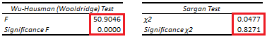
Below, we find examples of Wu-Hausman (Wooldridge) and Sargan tests auxiliary regressions F and chi-square tests from original multiple linear regression of house price explained by its lot size and number of bedrooms using whether house has a driveway and number of garage places as instrumental variables [3].
Courses
My online courses are hosted at Teachable website.
For more details on this concept, you can view my Linear Regression Courses.
References
[1] Durbin, James (1954). “Errors in variables”. Review of the International Statistical Institute. 22 (1/3): 23–32.
Wu, De-Min (1973). “Alternative Tests of Independence between Stochastic Regressors and Disturbances”. Econometrica. 41 (4): 733–750.
Hausman, J. A. (1978). “Specification Tests in Econometrics”. Econometrica. 46 (6): 1251–1271.
(Auxiliary linear regression test) Wooldridge JM (2010). “Econometric Analysis of Cross–Section and Panel Data”. 2nd edition. MIT Press. (Sec. 10.7.3.).
[2] Sargan, J. D. (1958). “The Estimation of Economic Relationships Using Instrumental Variables”. Econometrica. 26 (3): 393–415.
[3] Data Description: Sales prices of houses sold in the city of Windsor, Canada, during July, August and September, 1987.
Original Source: Anglin, P., and Gencay, R. (1996). Semiparametric Estimation of a Hedonic Price Function. Journal of Applied Econometrics, 11, 633–648.
Source: AER R Package HousePrices Object. Christian Kleiber and Achim Zeileis. (2008). Applied Econometrics with R. Springer-Verlag, New York.