Last Update: April 24, 2022
Exponential Smoothing is a forecasting method which flattens time series data. Brown Simple Exponential Smoothing Method [1] is used for forecasting time series data with no trend or seasonal patterns. It has an ETS(A,N,N) notation with additive errors and no trend or seasonal components.
As example, we can delimit univariate time series into training range
for model fitting and testing range
for model forecasting.
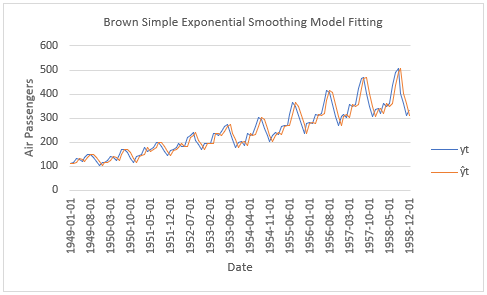
Then, we can fit model using Brown simple exponential smoothing method with formula . Training range model fitted values
are the one step ahead estimated
values and
is the level component with formula
. Training range level component fitted values
are the estimated
values and
is the level smoothing coefficient.
Training range model fitting can be done by estimating optimal level smoothing coefficient and optimal initial level fitted value
through minimizing sum of squared estimated model residuals with formula
. Training range estimated model residuals
with formula
are the differences between actual
and fitted
values. Notice that initial level fitted value
can also be estimated using simple formula [2].
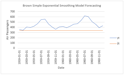
Next, we can forecast model using Brown simple exponential smoothing method with formula . Testing range model forecasted values
are the
steps ahead estimated
values and
is the last training range level component fitted value with formula
. Notice it is important to remember that when doing time series analysis and forecasting, past performance does not guarantee future results.
Below, we find example of model fitting and forecasting using Brown simple exponential smoothing method for airline passengers with training range as first ten years and testing range as last two years of data [3]. Optimal level smoothing coefficient and optimal initial level fitted value estimations done using Microsoft Excel® Solver® Add-in.
References
[1] Brown, Robert G. (1956). “Exponential Smoothing for Predicting Demand”. Cambridge, Massachusetts: Arthur D. Little Inc. p. 15.
[2] Hyndman, R.J., Koehler, A.B., Ord, J.K., Snyder, R.D. (2008). “Forecasting with exponential smoothing: the state space approach”, Springer-Verlag: New York.
[3] Data Description: Monthly international airline passenger numbers in thousands from 1949 to 1960.
Original Source: Box, G. E. P., Jenkins, G. M. and Reinsel, G. C. (1976). “Time Series Analysis, Forecasting and Control”. Third Edition. Holden-Day. Series G.
Source: datasets R Package AirPassengers Object. R Core Team (2021). “R: A language and environment for statistical computing”. R Foundation for Statistical Computing, Vienna, Austria.