Last Update: February 21, 2022
Heteroskedasticity is when linear regression errors have non-constant variance. This can be tested through Breusch-Pagan test [1] which evaluates whether model independent variables explain its errors variance. If model independent variables explain its errors variance, then model errors are assumed heteroskedastic or with non-constant variance. This can also be tested through White test [2] which evaluates whether model independent variables and squared independent variables explain its errors variance. If model independent variables and squared independent variables explain its errors variance, then model errors are assumed heteroskedastic or with non-constant variance.
As example, we can fit a three-variable multiple linear regression with formula . Then, we can obtain regression residuals
with formula
which are the estimated differences between actual
and fitted
values.
Next, we can do Breusch-Pagan test auxiliary regression with formula and chi-square test with joint null hypothesis that independent variables coefficients are equal to zero with formula
. If joint null hypothesis is rejected, then regression (1) errors are assumed heteroskedastic. Notice that null hypothesis test (4) can be done with an F-test.
After that, we can also do White test (no cross terms) auxiliary regression with formula and chi-square test with joint null hypothesis that independent variables and squared independent variables coefficients are equal to zero with formula
. If joint null hypothesis is rejected, then regression (1) errors are assumed heteroskedastic. Notice that null hypothesis test (6) can be done with an F-test.
Later, we can additionally do White test (cross terms) auxiliary regression with formula and chi-square test with joint null hypothesis that independent variables, squared independent variables and independent variables product coefficients are equal to zero with formula
. If joint null hypothesis is rejected, then regression (1) errors are assumed heteroskedastic and/or regression (1) has incorrect model equation specification. Notice that including independent variables products or cross terms to White test auxiliary regression (7) evaluates heteroskedasticity and model equation specification instead. Also, notice that null hypothesis test (8) can be done with an F-test.
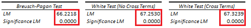
Below, we find examples of Breusch-Pagan, White (no cross terms) and White (cross terms) tests auxiliary regressions Lagrange Multiplier (LM) tests from original multiple linear regression of house price explained by its lot size and number of bedrooms [3].
Courses
My online courses are hosted at Teachable website.
For more details on this concept, you can view my Linear Regression Courses.
References
[1] Breusch, T. S.; Pagan, A. R. (1979). “A Simple Test for Heteroskedasticity and Random Coefficient Variation”. Econometrica. 47 (5): 1287–1294.
[2] White H (1980). “A Heteroskedasticity-Consistent Covariance Matrix Estimator and a Direct Test
for Heteroskedasticity.” Econometrica, 48(4), 817–838.
[3] Data Description: Sales prices of houses sold in the city of Windsor, Canada, during July, August and September, 1987.
Original Source: Anglin, P., and Gencay, R. (1996). Semiparametric Estimation of a Hedonic Price Function. Journal of Applied Econometrics, 11, 633–648.
Source: AER R Package HousePrices Object. Christian Kleiber and Achim Zeileis. (2008). Applied Econometrics with R. Springer-Verlag, New York.