Last Update: March 24, 2022
Instrumental Variables: Two Stage Least Squares estimation is used when linear regression independent variables are correlated with error term (endogenous).
As example, we can fit a three-variable original multiple linear regression with formula . Original linear regression fitted values
are the estimated
values,
is the endogenous independent variable (assumed correlated with original linear regression error term),
is the exogenous independent variable (assumed not correlated with original linear regression error term). Then, we can fit first stage least squares multiple linear regression with formula
. First stage least squares linear regression fitted values
are the estimated
values,
and
are the instrumental variables. Next, we can fit second stage least squares multiple linear regression with formula
. Second stage least squares linear regression fitted values
are the estimated
values. Notice that instrumental variables are not included within original linear regression, they are assumed correlated with endogenous independent variable and they are assumed not correlated with second stage least squares linear regression error term. Also, notice that stage by stage instead of simultaneous stages estimation of two stage least squares linear regression would estimate correct coefficients but incorrect standard errors and F-statistic. Additionally, notice that two stage least squares linear regression estimation assumes errors are homoskedastic unless heteroskedasticity consistent estimator is used.
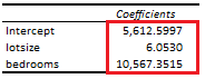
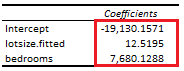
Below, we find an example of estimated coefficients comparison between original multiple linear regression of house price explained by its lot size and number of bedrooms and second stage least squares multiple linear regression of house price explained by its lot size first stage least squares multiple linear regression fitted values and number of bedrooms using whether house has a driveway and number of garage places as instrumental variables [1].
Courses
My online courses are hosted at Teachable website.
For more details on this concept, you can view my Linear Regression Courses.
References
[1] Data Description: Sales prices of houses sold in the city of Windsor, Canada, during July, August and September, 1987.
Original Source: Anglin, P., and Gencay, R. (1996). Semiparametric Estimation of a Hedonic Price Function. Journal of Applied Econometrics, 11, 633–648.
Source: AER R Package HousePrices Object. Christian Kleiber and Achim Zeileis. (2008). Applied Econometrics with R. Springer-Verlag, New York.