Last Update: February 21, 2022
Linear Regression: Coefficients Analysis is used to analyze linear relationship between one dependent variable and two or more independent variables
. Variable
is also known as target or response feature and variables
are also known as predictor features. It is also used to evaluate whether adding independent variables individually improved linear regression model.
As example, we can fit a three-variable multiple linear regression with formula . Regression fitted values
are the estimated
values. Estimated constant coefficient
is the
value when
and
. Estimated partial regression coefficient
is the estimated change in
when
changes in one unit while holding
constant. Similarly, estimated partial regression coefficient
is the estimated change in
when
changes in one unit while holding
constant.
Then, we can estimate coefficient standard error with formula
as squared root of residual mean squared error
multiplied by
element of matrix
principal diagonal.
Residual mean squared error with formula
is estimated as residual sum of squares
divided by residual degrees of freedom
. Residual sum of squares
with formula
is estimated as the sum of squared regression residuals
. Regression residuals
with formula
are estimated as differences between actual
and fitted
values. Residual degrees of freedom
with formula
are the number of observations
minus number of independent variables
minus constant term.
Matrix with dimension
x
is the inverse of the matrix product between the transpose of matrix
and matrix
. Matrix
with dimension
x
is the independent variables matrix including constant term column of ones.
Next, we can estimate coefficient t-statistic with formula
and do t-test with individual null hypothesis that independent variable
coefficient is equal to zero with formula
. If individual null hypothesis is rejected, then adding independent variable
improved linear regression model.
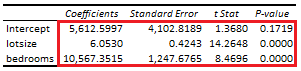
Below, we find an example of coefficients analysis from multiple linear regression of house price explained by its lot size and number of bedrooms [1].
Courses
My online courses are hosted at Teachable website.
For more details on this concept, you can view my Linear Regression Courses.
References
[1] Data Description: Sales prices of houses sold in the city of Windsor, Canada, during July, August and September, 1987.
Original Source: Anglin, P., and Gencay, R. (1996). Semiparametric Estimation of a Hedonic Price Function. Journal of Applied Econometrics, 11, 633–648.
Source: AER R Package HousePrices Object. Christian Kleiber and Achim Zeileis. (2008). Applied Econometrics with R. Springer-Verlag, New York.