Last Update: February 21, 2022
Simple linear regression is used to model linear relationship between two variables and
. Dependent variable
is the explained one which is also known as target or response feature. Independent variable
is the explanatory one which is also known as predictor feature.
When doing simple linear regression, we can start by drawing a scatter chart with variables and
on the vertical and horizontal axis, respectively. Then, we can draw a line which describes linear relationship between variables
and
. This line represents model fitting with formula
. Notice that we are using ˄ or hat character in formula notation because they are estimates. Regression fitted values
are the estimated
values. Estimated constant or intercept coefficient
is the
value when
or the
value where line crosses vertical axis. Estimated slope coefficient
is the estimated change in
when
changes in one unit.
Model fitting can be done using ordinary least squares method with formula . This method minimizes the sum of squared estimated regression residuals
. Estimated regression residuals
with formula
are the differences between actual
and fitted
values.
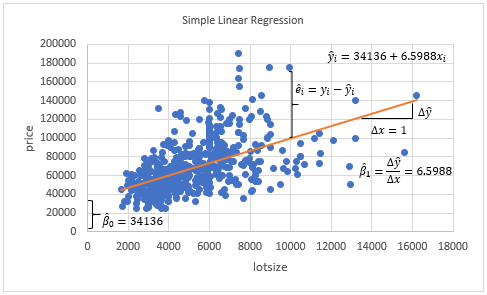
Below, we find an example of scatter chart with simple linear regression of house price explained by its lot size [1].
Courses
My online courses are hosted at Teachable website.
For more details on this concept, you can view my Linear Regression Courses.
References
[1] Data Description: Sales prices of houses sold in the city of Windsor, Canada, during July, August and September, 1987.
Original Source: Anglin, P., and Gencay, R. (1996). Semiparametric Estimation of a Hedonic Price Function. Journal of Applied Econometrics, 11, 633–648.
Source: AER R package HousePrices object. Christian Kleiber and Achim Zeileis. (2008). Applied Econometrics with R. Springer-Verlag, New York.