Time Series Decomposition: Classical Method

Last Update: June 1, 2022

Time Series Decomposition: Classical Method is used to estimate time series trend-cycle, seasonal and remainder components.

As example, we can delimit univariate time series  into training range  for model fitting and testing range  for model forecasting.

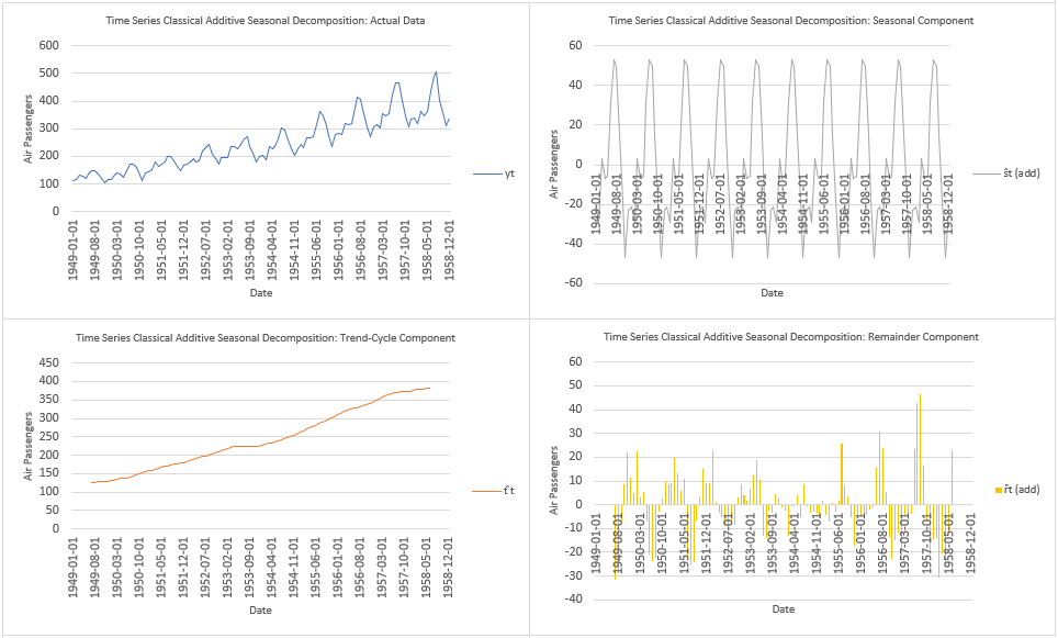
Then, we can do training range univariate time series classical additive seasonal decomposition by moving averages trend-cycle, seasonal and remainder components estimation. Notice that we have to evaluate whether time series classical additive or multiplicative seasonal decomposition is needed.

Next, we estimate trend-cycle component with formulas  when seasonal period  is an even number and  when seasonal period  is an odd number. As example, with monthly data, . Training range trend-cycle component estimated values  are the two periods averages of univariate time series centered seasonal simple moving averages when seasonal period  is an even number and the univariate time series centered seasonal simple moving averages when seasonal period  is an odd number. Training range univariate time series centered seasonal simple moving averages  are the  rolling averages with formulas  where  when seasonal period  is an even number and  where  when seasonal period  is an odd number. After that we estimate detrended univariate time series values with formula .

Later, we estimate seasonal component with formula . Training range seasonal component estimated values  are the estimated seasonal index values  adjusted so that they add to zero. As example, with monthly data, we estimate December seasonal index with formula  where  is the number of December detrended univariate time series values within training range. Training range December seasonal index value  is the average of all estimated December detrended univariate time series values.

Then we estimate remainder component with formula . Training range remainder component estimated values  are the  values minus estimated trend-cycle component values  minus estimated seasonal component values .

Below, we find example of training range univariate time series classical additive seasonal decomposition by moving averages using airline passengers data [1]. Training range as first ten years and testing range as last two years of data.

References

Data Description: Monthly international airline passenger numbers in thousands from 1949 to 1960.

Original Source: Box, G. E. P., Jenkins, G. M. and Reinsel, G. C. (1976). “Time Series Analysis, Forecasting and Control”. Third Edition. Holden-Day. Series G.

Source: datasets R Package AirPassengers Object. R Core Team (2021). “R: A language and environment for statistical computing”. R Foundation for Statistical Computing, Vienna, Austria.