Last Update: February 21, 2022
Multicollinearity in Python can be tested using statsmodels package variance_inflation_factor function found within statsmodels.stats.outliers_influence module for estimating multiple linear regression independent variables variance inflation factors individually. Main parameters within variance_inflation_factor function are exog with matrix of independent variables values and exog_idx with column index of independent variable for its variance inflation factor estimation. Independent variables variance inflation factors can also be estimated as main diagonal values from their inverse correlation matrix using numpy package inv function found within numpy.linalg module. Main parameter within inv function is a with matrix to be inverted.
As example, we can test multicollinearity of independent variables from multiple linear regression of house price explained by its lot size, number of bedrooms, bathrooms and stories using data included within AER R package HousePrices object [1].
First, we import packages numpy for estimating inverse correlation matrix, pandas for data frame objects creation, seaborn for inverse correlation matrix chart and statsmodels for data downloading, adding constant column to independent variables data frame and estimating variance inflation factors individually [2].
In [1]:
import numpy as np
import pandas as pd
import seaborn as sns
import statsmodels.api as sm
import statsmodels.tools.tools as smt
import statsmodels.stats.outliers_influence as smo
Second, we create houseprices data object using get_rdataset function and display first five rows and five columns of data using print function and head data frame method to view its structure.
In [2]:
houseprices = sm.datasets.get_rdataset(dataname="HousePrices", package="AER", cache=True).data
print(houseprices.iloc[:, 0:5].head())
Out [2]:
     price  lotsize  bedrooms  bathrooms  stories
0  42000.0     5850         3          1        2
1  38500.0     4000         2          1        1
2  49500.0     3060         3          1        1
3  60500.0     6650         3          1        2
4  61000.0     6360         2          1        1
Third, we create independent variables data frame subset stored within ivar object and display first five rows of data using print function and head data frame method to view its structure.
In [3]:
ivar = houseprices.iloc[:, 1:5]
print(ivar.head())
Out [3]:
   lotsize  bedrooms  bathrooms  stories
0     5850         3          1        2
1     4000         2          1        1
2     3060         3          1        1
3     6650         3          1        2
4     6360         2          1        1
Fourth, we add a constant column to independent variables data frame using add_constant function and store outcome within ivarc object. Within add_constant function, parameters data=ivar includes matrix of independent variables and prepend=False includes logical value to add constant at last column of matrix. Next, we can print independent variables estimated variance inflation factors individually using variance_inflation_factor function. Within variance_inflation_factor function, parameters exog=ivarc.values includes matrix of independent variables values and exog_idx=0 includes column index of lotsize independent variable for its variance inflation factor estimation as an example.
In [4]:
ivarc = smt.add_constant(data=ivar, prepend=False)
vif_lotsize = smo.variance_inflation_factor(exog=ivarc.values, exog_idx=0)
print(vif_lotsize)
Out [4]:
1.047054041442195
Fifth, we can print independent variables estimated variance inflation factors as main diagonal values from their inverse correlation matrix using inv function and store outcome within ivaricor object as DataFrame. Within inv function, parameter a = ivar.corr() includes independent variables estimated correlation matrix using corr data frame function. Within DataFrame function, parameters data=ivaricor includes independent variables previously estimated inverse correlation matrix, index=ivar.columns includes matrix rows names and columns=ivar.columns includes matrix columns names.
In [5]:
ivaricor = np.linalg.inv(a = ivar.corr())
ivaricor = pd.DataFrame(data=ivaricor, index=ivar.columns, columns=ivar.columns)
print(ivaricor)
Out [5]:
            lotsize  bedrooms  bathrooms   stories
lotsize    1.047054 -0.099092  -0.168300  0.007355
bedrooms  -0.099092  1.310851  -0.335344 -0.417828
bathrooms -0.168300 -0.335344   1.239203 -0.250689
stories    0.007355 -0.417828  -0.250689  1.251087
Sixth, we can additionally visualize independent variables estimated variance inflation factors as main diagonal values from their inverse correlation matrix chart using seaborn package heatmap function. Within heatmap function, parameters data=ivaricor includes matrix to visualize, cmap="Blues" includes matplotlib package colormap name and annot=True includes logical value to write the data value in each cell.
In [6]:
sns.heatmap(data=ivaricor, cmap="Blues", annot=True)
Out [6]: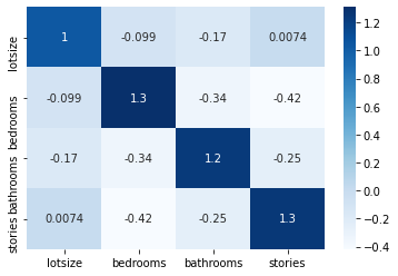
Courses
My online courses are hosted at Teachable website.
For more details on this concept, you can view my Linear Regression in Python Course.
References
[1] Data Description: Sales prices of houses sold in the city of Windsor, Canada, during July, August and September, 1987.
Original Source: Anglin, P., and Gencay, R. (1996). Semiparametric Estimation of a Hedonic Price Function. Journal of Applied Econometrics, 11, 633–648.
[2] numpy Python package: Travis E. Oliphant, et al. (2020). Array programming with NumPy. Nature, 585, 357–362.
pandas Python package: Wes McKinney. (2010). Data Structures for Statistical Computing in Python, Proceedings of the 9th Python in Science Conference, 51-56.
seaborn Python package: Waskom, M. L., (2021). “seaborn: statistical data visualization”. Journal of Open Source Software, 6(60), 3021.
statsmodels Python package: Seabold, Skipper, and Josef Perktold. (2010). “statsmodels: Econometric and statistical modeling with python.” Proceedings of the 9th Python in Science Conference.