Last Update: February 21, 2022
Normality in Error Term: Q-Q Plot in Python can be done using statsmodels package qqplot function found within statsmodels.api module and matplotlib package plot function found within matplotlib.pyplot module for evaluating whether points comparing linear regression residuals sample quantiles and normal distribution theoretical quantiles are within quantiles regression line fit. Main parameters within qqplot function are data with model residuals, dist with comparison probability distribution and line with quantiles regression line fit, regression line fit, standardized line or 45-degree line options.
Normality in Error Term: Jarque-Bera Test in Python can be done using statsmodels package jarque_bera function found within statsmodels.stats.api module for evaluating whether linear regression residuals skewness and excess kurtosis are equal to zero. Main parameter within jarque_bera function is resid with model residuals.
As example, we can do residuals Q-Q plot and Jarque-Bera test from multiple linear regression of house price explained by its lot size and number of bedrooms using data included within AER R package HousePrices object [1].
First, we import statsmodels package for data downloading, multiple linear regression fitting, Q-Q plot and Jarque-Bera test, scipy package for normal probability distribution and matplotlib for Q-Q plot [2].
In [1]:
import statsmodels.api as sm
import statsmodels.formula.api as smf
import statsmodels.stats.api as sms
import scipy.stats as st
import matplotlib.pyplot as plt
Second, we create houseprices data object using get_rdataset function and display first five rows and three columns of data using print function and head data frame method to view its structure.
In [2]:
houseprices = sm.datasets.get_rdataset(dataname="HousePrices", package="AER", cache=True).data
print(houseprices.iloc[:, 0:3].head())
Out [2]:
     price  lotsize  bedrooms
0  42000.0     5850         3
1  38500.0     4000         2
2  49500.0     3060         3
3  60500.0     6650         3
4  61000.0     6360         2
Third, we fit multiple linear regression with ols function using variables within houseprices data object and store results within mlr object. Within ols function, parameter formula="price ~ lotsize + bedrooms" fits model where house price is explained by its lot size and number of bedrooms.
In [3]:
mlr = smf.ols(formula="price ~ lotsize + bedrooms", data=houseprices).fit()
Fourth, we get residuals from mlr multiple linear regression results object and store them within res object.
In [4]:
res = mlr.resid
Fifth, we do normal Q-Q plot using qqplot and plot functions. Within qqplot function, parameters data=res includes model residuals, dist=st.norm includes scipy package normal probability distribution for comparison and line="q" includes quantiles regression line fit.
In [5]:
fig = sm.qqplot(data=res, dist=st.norm, line="q")
plt.title("Normal Q-Q Plot")
plt.show()
Out [5]: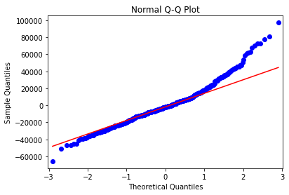
Figure 1. Residuals normal Q-Q plot from multiple linear regression of house price explained by its lot size and number of bedrooms.Sixth, we do Jarque-Bera test using jarque_bera function, store results within jbtest object and print its JB test statistic and JBpv test statistic p-value results. Within jarque_bera function, parameter resids = res includes model residuals.
In [6]:
jbtest = sms.jarque_bera(resids = res)
print("JB:", jbtest[0], "JBpv:", jbtest[1])
Out [6]:
JB: 146.85443903231146 JBpv: 1.2911114798088417e-32
Courses
My online courses are hosted at Teachable website.
For more details on this concept, you can view my Linear Regression in Python Course.
References
[1] Data Description: Sales prices of houses sold in the city of Windsor, Canada, during July, August and September, 1987.
Original Source: Anglin, P., and Gencay, R. (1996). Semiparametric Estimation of a Hedonic Price Function. Journal of Applied Econometrics, 11, 633–648.
[2] statsmodels Python package: Seabold, Skipper, and Josef Perktold. (2010). “statsmodels: Econometric and statistical modeling with python”. Proceedings of the 9th Python in Science Conference.
scipy Python package: Pauli Virtanen, Ralf Gommers, Travis E. Oliphant, Matt Haberland, Tyler Reddy, David Cournapeau, Evgeni Burovski, Pearu Peterson, Warren Weckesser, Jonathan Bright, Stéfan J. van der Walt, Matthew Brett, Joshua Wilson, K. Jarrod Millman, Nikolay Mayorov, Andrew R. J. Nelson, Eric Jones, Robert Kern, Eric Larson, CJ Carey, İlhan Polat, Yu Feng, Eric W. Moore, Jake VanderPlas, Denis Laxalde, Josef Perktold, Robert Cimrman, Ian Henriksen, E.A. Quintero, Charles R Harris, Anne M. Archibald, Antônio H. Ribeiro, Fabian Pedregosa, Paul van Mulbregt, and SciPy 1.0 Contributors. (2020). SciPy 1.0: Fundamental Algorithms for Scientific Computing in Python. Nature Methods, 17(3), 261-272.
matplotlib Python package: John D. Hunter. (2007). Matplotlib: A 2D Graphics Environment. Computing in Science & Engineering, 9, 90-95.