Last Update: February 21, 2022
Simple linear regression in Python can be fitted using statsmodels package ols function found within statsmodels.formula.api module. Main parameters within ols function are formula with “y ~ x” model description string and data with data frame object including model variables. Therefore, ols(formula = “y ~ x”, data = model_data).fit() code line fits model using variables included within
model_data object.
As example, we can fit simple linear regression of house price explained by its lot size using data included within AER R package HousePrices object [1].
First, we import packages statsmodels for data downloading, model fitting and seaborn for charting [2].
In [1]:
import statsmodels.api as sm
import statsmodels.formula.api as smf
import seaborn as sns
Second, we create houseprices data object using get_rdataset function and display first five rows and two columns of data using print function and head data frame method to view its structure.
In [2]:
houseprices = sm.datasets.get_rdataset(dataname="HousePrices", package="AER", cache=True).data
print(houseprices.iloc[:, 0:2].head())
Out[2]:
price lotsize
0 42000.0 5850
1 38500.0 4000
2 49500.0 3060
3 60500.0 6650
4 61000.0 6360Third, we draw scatter chart with regression line colored in red which doesn’t display its confidence interval.
In [3]:
sns.regplot(x="lotsize", y="price", data=houseprices, ci=None, line_kws={"color": "red"})
Out [3]: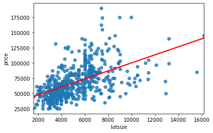
Figure 1. Simple linear regression scatter chart of house price explained by its lot size.Fourth, we fit model with ols function using variables within houseprices data object, store outcome within slr object and print its params parameter to observe coefficients estimates. Within ols function, parameter formula = “price ~ lotsize” fits model where house price is explained by its lot size.
In [4]:
slr = smf.ols(formula="price ~ lotsize", data=houseprices).fit()
print(slr.params)
Out [4]:
Intercept 34136.191565
lotsize 6.598768
dtype: float64Courses
My online courses are hosted at Teachable website.
For more details on this concept, you can view my Linear Regression in Python Course.
References
[1] Data Description: Sales prices of houses sold in the city of Windsor, Canada, during July, August and September, 1987.
Original Source: Anglin, P., and Gencay, R. (1996). Semiparametric Estimation of a Hedonic Price Function. Journal of Applied Econometrics, 11, 633–648.
[2] Seabold, Skipper, and Josef Perktold. (2010). “statsmodels: Econometric and statistical modeling with python.” Proceedings of the 9th Python in Science Conference.
Waskom, M. L., (2021). “seaborn: statistical data visualization”. Journal of Open Source Software, 6(60), 3021.