Last Update: April 24, 2022
Exponential Smoothing: Brown Simple Method in R can be done using forecast package ses function for forecasting by flattening time series data with no trend or seasonal patterns. Main parameters within ses function are y with time series data, h with number of forecasting periods, PI with logical value on whether prediction intervals are estimated, level with prediction intervals statistical confidence levels and initial with initial state values estimation method.
As example, we can do model fitting and forecasting using Brown simple exponential smoothing method for airline passengers with training range as first ten years and testing range as last two years using data included within datasets package AirPassengers object [1].
First, we load packages forecast for Brown simple exponential smoothing method and ggplot2 for its chart [2].
In [1]:
library(forecast)
library(ggplot2)
Second, we create mdata model data object copied from datasets package AirPassengers object and print first six months of data using head function to view time series object structure.
In [2]:
mdata <- AirPassengers
head(mdata)
Out [2]:
     Jan Feb Mar Apr May Jun
1949 112 118 132 129 121 135
Third, we delimit training range for model fitting as first ten years of data with window function and store outcome within tdata object. Within window function, parameters x = mdata includes full range model data and end = c(1958, 12) includes training range end time. Then, we delimit testing range for model forecasting as last two years of data with window function and store outcome within fdata object. Within window function, parameters x = mdata includes full range model data and start = c(1959, 1) includes training range start time. Notice that training and testing ranges delimiting was only included as an educational example which can be modified according to your needs.
In [3]:
tdata <- window(x = mdata, end = c(1958, 12))
fdata <- window(x = mdata, start = c(1959, 1))
Fourth, we fit and forecast Brown simple exponential smoothing method with ses function using tdata training range data object and store outcome within brown object. Within ses function, parameters y = tdata includes training range data, h = 24 includes twenty four months or two years forecasting period, PI = TRUE includes logical value to estimate prediction intervals, level = c(80, 95) includes prediction intervals eighty and ninety five percent statistical confidence levels and initial = "optimal" includes optimized initial state values. Notice that initial state values can also be estimated using simple formula. Also, notice that ses function parameters were only included as educational examples which can be modified according to your needs. Additionally, notice it is important to remember that when doing time series analysis and forecasting, past performance does not guarantee future results.
In [4]:
brown <- ses(y = tdata, h = 24, PI = TRUE, level = c(80, 95),
             initial = "optimal")
Fifth, we view Brown simple exponential smoothing method forecast with autoplot, autolayer and labs functions. Within autoplot function, parameter object = brown includes brown forecast object. Within autolayer function, parameters object = fdata includes testing range data object, color = "black" includes line color and linetype = 2 includes dashed line type. Within labs function, parameters y = "Air Passengers" includes vertical axis label and x = "Year" includes horizontal axis label.
In [5]:
autoplot(object = brown) +
  autolayer(object = fdata, color = "black", linetype = 2) +
  labs(y = "Air Passengers", x = "Year")
Out [5]: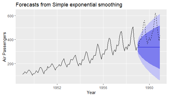
Figure 1. Model fitting and forecasting using Brown simple exponential smoothing method for airline passengers with training range as first ten years and testing range as last two years of data.References
[1] Data Description: Monthly international airline passenger numbers in thousands from 1949 to 1960.
Original Source: Box, G. E. P., Jenkins, G. M. and Reinsel, G. C. (1976). “Time Series Analysis, Forecasting and Control”. Third Edition. Holden-Day. Series G.
Source: datasets R Package AirPassengers Object. R Core Team (2021). “R: A language and environment for statistical computing”. R Foundation for Statistical Computing, Vienna, Austria.
[2] forecast R Package. Hyndman R, Athanasopoulos G, Bergmeir C, Caceres G, Chhay L,
O’Hara-Wild M, Petropoulos F, Razbash S, Wang E, Yasmeen F (2022). “forecast: Forecasting functions for time series and linear models”. R package version 8.16
ggplot2 R Package. Hadley Wickham (2016). “ggplot2: Elegant Graphics for Data Analysis”. Springer-Verlag New York