Last Update: February 21, 2022
Multicollinearity in R can be tested using car package vif function for estimating multiple linear regression independent variables variance inflation factors. Main parameter within vif function is mod with previously fitted lm model. Independent variables variance inflation factors can also be estimated as main diagonal values from their inverse correlation matrix using MASS package ginv function. Main parameter within ginv function is X with independent variables previously estimated correlation matrix using stats package cor function.
As example, we can test multicollinearity of independent variables from multiple linear regression of house price explained by its lot size, number of bedrooms, bathrooms and stories using data included within AER package HousePrices object [1].
First, we load packages AER for data, car for estimating variance inflation factors, MASS for estimating inverse correlation matrix and corrplot for inverse correlation matrix chart [2].
In [1]:
library(AER)
library(car)
library(MASS)
library(corrplot)
Second, we create HousePrices data object from AER package using data function and print first six rows and five columns of data using head function to view data.frame structure.
In [2]:
data(HousePrices)
head(HousePrices[, 1:5])
Out [2]:
  price lotsize bedrooms bathrooms stories
1 42000    5850        3         1       2
2 38500    4000        2         1       1
3 49500    3060        3         1       1
4 60500    6650        3         1       2
5 61000    6360        2         1       1
6 66000    4160        3         1       1
Third, we can fit multiple linear regression model using lm function and store outcome within mlr object. Within lm function, parameter formula = price ~ lotsize + bedrooms + bathrooms + stories fits model where house price is explained by its lot size, number of bedrooms, bathrooms and stories. Then, we can print independent variables estimated variance inflation factors using vif function. Within vif function, parameter mod = mlr includes previously fitted lm model.
In [3]:
mlr <- lm(formula = price ~ lotsize + bedrooms + bathrooms + stories, data = HousePrices)
vif(mod = mlr)
Out [3]:
  lotsize  bedrooms bathrooms   stories
 1.047054  1.310851  1.239203  1.251087
Fourth, we can create independent variables data frame subset and store it within ivar object. Next, we can also print independent variables estimated variance inflation factors as main diagonal values from their inverse correlation matrix using ginv function and store outcome within ivaricor object. Within ginv function, parameter X = cor(ivar) includes independent variables estimated correlation matrix using cor function.
In [4]:
ivar <- HousePrices[, 2:5]
ivaricor <- ginv(X = cor(ivar))
colnames(ivaricor) <- colnames(ivar)
rownames(ivaricor) <- colnames(ivar)
ivaricor
Out [4]:
               lotsize    bedrooms  bathrooms      stories
lotsize    1.047054041 -0.09909201 -0.1683001  0.007354973
bedrooms  -0.099092014  1.31085130 -0.3353444 -0.417827752
bathrooms -0.168300120 -0.33534441  1.2392031 -0.250688885
stories    0.007354973 -0.41782775 -0.2506889  1.251086952
Fifth, we can additionally visualize independent variables estimated variance inflation factors as main diagonal values from their inverse correlation matrix chart using corrplot package corrplot function. Within corrplot function, parameters corr = ivaricor includes matrix to visualize, method = "number" includes visualization method to be used and is.corr = FALSE includes logical value that input matrix is an inverse correlation matrix and not a correlation matrix.
In [5]:
corrplot(corr = ivaricor, method = "number", is.corr = FALSE)
Out [5]: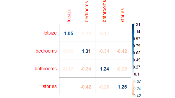
Courses
My online courses are hosted at Teachable website.
For more details on this concept, you can view my Linear Regression in R Course.
References
[1] Data Description: Sales prices of houses sold in the city of Windsor, Canada, during July, August and September, 1987.
Original Source: Anglin, P., and Gencay, R. (1996). Semiparametric Estimation of a Hedonic Price Function. Journal of Applied Econometrics, 11, 633–648.
[2] AER R Package: Christian Kleiber and Achim Zeileis. (2008). Applied Econometrics with R. Springer-Verlag, New York.
car R Package: John Fox and Sanford Weisberg. (2019). An R Companion to Applied Regression. Third Edition. Sage, Thousand Oaks, CA.
MASS R Package: W. N. Venables and B. D. Ripley. (2002). Modern Applied Statistics with S. Fourth Edition. Springer, New York.
corrplot R Package: Taiyun Wei and Viliam Simko. (2021). R package ‘corrplot’: Visualization of a Correlation Matrix. Version 0.90.