Last Update: February 21, 2022
Normality in Error Term: Q-Q Plot in R can be done using ggplot2 package ggplot, stat_qq and stat_qq_line functions for evaluating whether points comparing linear regression residuals sample quantiles and normal distribution theoretical quantiles are within quantiles regression line fit. Main parameters within ggplot function are data with model residuals data frame and aes with variables aesthetic mappings. Main parameter within stat_qq function is distribution with probability distribution quantile function to use. Main parameters within stat_qq_line function are distribution with probability distribution quantile function to use and line.p with percentiles vector for fitting quantiles regression line.
Normality in Error Term: Jarque-Bera Test can be done using tseries package jarque.bera.test function for evaluating whether linear regression residuals skewness and excess kurtosis are equal to zero. Main parameter within jarque.bera.test function is x with model residuals numeric vector.
As example, we can do residuals Q-Q plot and Jarque-Bera test from multiple linear regression of house price explained by its lot size and number of bedrooms using data included within AER package HousePrices object [1].
First, we load packages AER for data, ggplot2 for Q-Q plot and tseries for Jarque-Bera test [2].
In [1]:
library(AER)
library(ggplot2)
library(tseries)
Second, we create HousePrices data object from AER package using data function and print first six rows and three columns of data using head function to view data.frame structure.
In [2]:
data(HousePrices)
head(HousePrices[, 1:3])
Out [2]:
  price lotsize bedrooms
1 42000    5850        3
2 38500    4000        2
3 49500    3060        3
4 60500    6650        3
5 61000    6360        2
6 66000    4160        3
Third, we fit multiple linear regression using lm function and store results within mlr object. Within lm function, parameter formula = price ~ lotsize + bedrooms fits model where house price is explained by its lot size and number of bedrooms.
In [3]:
mlr <- lm(formula = price ~ lotsize + bedrooms, data = HousePrices)
Fourth, we get residuals from mlr multiple linear regression object and store them within res object.
In [4]:
res <- mlr$residuals
Fifth, we do normal Q-Q plot using ggplot, stat_qq and stat_qq_line functions. Within ggplot function, parameters data = data.frame(res) includes residuals as data.frame and aes(sample = res) includes residuals data variable sample aesthetics mapping required by stat_qq function. Within stat_qq function, parameter distribution = qnorm includes normal distribution quantile function. Within stat_qq_line function, parameters distribution = qnorm includes normal distribution quantile function and line.p = c(0.25, 0.75) includes 0.25 and 0.75 percentiles vector for fitting quantiles regression line.
In [5]:
ggplot(data = data.frame(res), aes(sample = res)) +
  stat_qq(distribution = qnorm) +
  stat_qq_line(distribution = qnorm, line.p = c(0.25, 0.75), color = "red") +
  labs(title = "Normal Q-Q Plot", x = "Theoretical Quantiles", y = "Sample Quantiles")
Out [5]: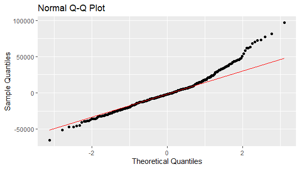
Figure 1. Residuals normal Q-Q plot from multiple linear regression of house price explained by its lot size and number of bedrooms.Sixth, we do Jarque-Bera test using jarque.bera.test function. Within jarque.bera.test function, parameter x = res includes residuals numeric vector.
In [6]:
jarque.bera.test(x = res)
Out [6]:
	Jarque Bera Test

data:  res
X-squared = 146.85, df = 2, p-value < 2.2e-16
Courses
My online courses are hosted at Teachable website.
For more details on this concept, you can view my Linear Regression in R Course.
References
[1] Data Description: Sales prices of houses sold in the city of Windsor, Canada, during July, August and September, 1987.
Original Source: Anglin, P., and Gencay, R. (1996). Semiparametric Estimation of a Hedonic Price Function. Journal of Applied Econometrics, 11, 633–648.
[2] AER R Package: Christian Kleiber and Achim Zeileis. (2008). Applied Econometrics with R. Springer-Verlag, New York.
ggplot2 R Package: Hadley Wickham. (2016). ggplot2: Elegant Graphics for Data Analysis. Springer-Verlag New York.
tseries R Package: Adrian Trapletti and Kurt Hornik. (2020). tseries: Time Series Analysis and Computational Finance. R package version 0.10-48.