Last Update: February 21, 2022
Simple linear regression in R can be fitted using stats package lm function. Main parameters within lm function are formula with y ~ x model description and data with data.frame object including model variables. Therefore, lm(y ~ x, data = model.data) code line fits model using variables included within
model.data object.
As example, we can fit simple linear regression of house price explained by its lot size using data included within AER package HousePrices object [1].
First, we load packages AER for data and ggplot2 for charting [2].
In [1]:
library(AER)
library(ggplot2)
Second, we create HousePrices data object from AER package using data function and print first six rows and two columns of data using head function to view data.frame structure.
In [2]:
data(HousePrices)
head(HousePrices[,1:2])
Out [2]:
price lotsize
1 42000 5850
2 38500 4000
3 49500 3060
4 60500 6650
5 61000 6360
6 66000 4160Third, we draw scatter chart with regression line which doesn’t display its confidence interval.
In [3]:
ggplot(data = HousePrices, aes(x = lotsize, y = price)) +
  geom_point() +
  geom_smooth(method = "lm", se = FALSE)
Out [3]: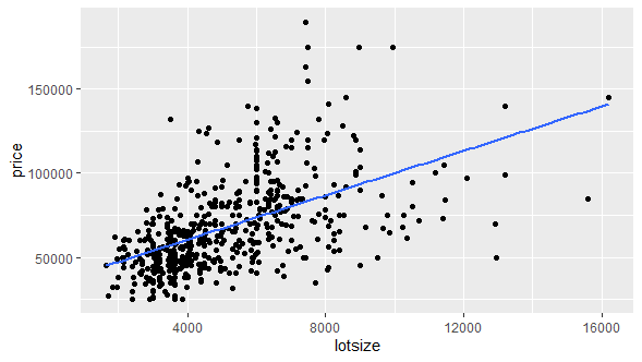
Figure 1. Simple linear regression scatter chart of house price explained by its lot size.Fourth, we fit model with lm function using variables within HousePrices data object, store outcome within slr object and print its coefficients estimates. Within lm function, parameter formula = price ~ lotsize fits model where house price is explained by its lot size.
In [4]:
slr <- lm(formula = price ~ lotsize, data = HousePrices)
slr
Out [4]:
Call:
lm(formula = price ~ lotsize, data = HousePrices)
Coefficients:
(Intercept) lotsize
34136.192 6.599Courses
My online courses are hosted at Teachable website.
For more details on this concept, you can view my Linear Regression in R Course.
References
[1] Data Description: Sales prices of houses sold in the city of Windsor, Canada, during July, August and September, 1987.
Original Source: Anglin, P., and Gencay, R. (1996). Semiparametric Estimation of a Hedonic Price Function. Journal of Applied Econometrics, 11, 633–648.
[2] AER R Package. Christian Kleiber and Achim Zeileis. (2008). Applied Econometrics with R. Springer-Verlag, New York.
ggplot2 R Package. Hadley Wickham (2016). ggplot2: Elegant Graphics for Data Analysis. Springer-Verlag, New York.