Stationarity: Augmented Dickey-Fuller Test in R

Last Update: May 13, 2022

Stationarity: Augmented Dickey-Fuller Test in R can be done using tseries package adf.test function for evaluating whether time series mean does not change over time. Main parameters within adf.test function are x with time series data, alternative with alternative hypothesis string and k with lag order to calculate test statistic.

As example, we can do training range augmented Dickey-Fuller test using data included within datasets package AirPassengers object [1].

First, we load packages forecast for time series characteristics, ggplot2 for training range chart and tseries for augmented Dickey-Fuller test [2].

In [1]:
library(forecast)
library(ggplot2)
library(tseries)

Second, we create mdata model data object copied from datasets package AirPassengers object and print first six months of data using head function to view time series object structure.

In [2]:
mdata <- AirPassengers
head(mdata)

Out [2]:
     Jan Feb Mar Apr May Jun
1949 112 118 132 129 121 135

Third, we delimit training range for model fitting as first ten years of data with window function and store outcome within tdata object. Within window function, parameters x = mdata includes full range model data and end = c(1958, 12) includes training range end time. Then, we delimit testing range for model forecasting as last two years of data with window function and store outcome within fdata object. Within window function, parameters x = mdata includes full range model data and start = c(1959, 1) includes training range start time. Notice that training and testing ranges delimiting was only included as an educational example which can be modified according to your needs.

In [3]:
tdata <- window(x = mdata, end = c(1958, 12))
fdata <- window(x = mdata, start = c(1959, 1))

Fourth, we view training range data with autoplot and labs functions. Within autoplot function, parameter object = tdata includes training range data object. Within labs function, parameters y = "Air Passengers" includes vertical axis label and x = "Year" includes horizontal axis label.

In [4]:
autoplot(object = tdata) + labs(y = "Air Passengers", x = "Year")

Out [4]: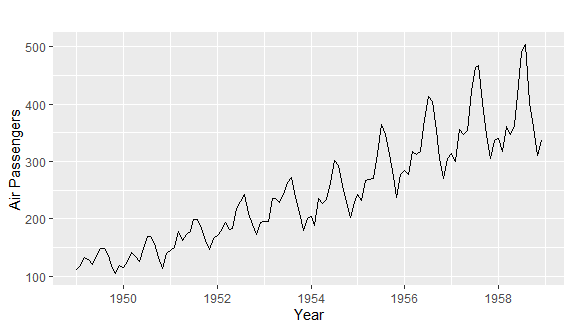

Fifth, we do training range data augmented Dickey-Fuller test with adf.test function. Within adf.test function, parameters x = tdata includes training range data object, alternative = "stationary" includes stationary alternative hypothesis string and k = 12 includes twelve lags of training range values differences to calculate test statistic. Notice that adf.test function includes constant and deterministic linear trend variable by default within test regression. Also, notice that we have to test whether constant, deterministic linear trend variable and which training range values differences number of lags are needed within test regression.

In [5]:
adf.test(x = tdata, alternative = "stationary", k = 12)

Out [5]:
	Augmented Dickey-Fuller Test

data:  tdata
Dickey-Fuller = -1.8449, Lag order = 12, p-value = 0.641
alternative hypothesis: stationary

References

[1] Data Description: Monthly international airline passenger numbers in thousands from 1949 to 1960.

Original Source: Box, G. E. P., Jenkins, G. M. and Reinsel, G. C. (1976). “Time Series Analysis, Forecasting and Control”. Third Edition. Holden-Day. Series G.

Source: datasets R Package AirPassengers Object. R Core Team (2021). “R: A language and environment for statistical computing”. R Foundation for Statistical Computing, Vienna, Austria.

[2] forecast R Package. Hyndman R, Athanasopoulos G, Bergmeir C, Caceres G, Chhay L,
O’Hara-Wild M, Petropoulos F, Razbash S, Wang E, Yasmeen F (2022). “forecast: Forecasting functions for time series and linear models”. R package version 8.16

ggplot2 R Package. Hadley Wickham (2016). “ggplot2: Elegant Graphics for Data Analysis”. Springer-Verlag New York

tseries R Package: Adrian Trapletti and Kurt Hornik (2021). “tseries: Time Series Analysis and Computational Finance”. R package version 0.10-49.