Last Update: June 20, 2022
Time Series Decomposition: Classical Method in R can be done using stats package decompose function for estimating time series trend-cycle, seasonal and remainder components. Main parameters within decompose function are x with time series data, type with seasonal component type and filter with vector of seasonal component filter coefficients.
As example, we can do training range univariate time series classical additive seasonal decomposition by moving averages using data included within datasets package AirPassengers object [1].
First, we load packages forecast for time series characteristics, ggplot2 for training range and time series decomposition charts [2].
In [1]:
library(forecast)
library(ggplot2)
Second, we create mdata model data object copied from datasets package AirPassengers object and print first six months of data using head function to view time series object structure.
In [2]:
mdata <- AirPassengers
head(mdata)
Out [2]:
     Jan Feb Mar Apr May Jun
1949 112 118 132 129 121 135
Third, we delimit training range for model fitting as first ten years of data with window function and store outcome within tdata object. Within window function, parameters x = mdata includes full range model data and end = c(1958, 12) includes training range end time. Then, we delimit testing range for model forecasting as last two years of data with window function and store outcome within fdata object. Within window function, parameters x = mdata includes full range model data and start = c(1959, 1) includes training range start time. Notice that training and testing ranges delimiting was only included as an educational example which can be modified according to your needs.
In [3]:
tdata <- window(x = mdata, end = c(1958, 12))
fdata <- window(x = mdata, start = c(1959, 1))
Fourth, we view training range data with autoplot and labs functions. Within autoplot function, parameter object = tdata includes training range data object. Within labs function, parameters y = "Air Passengers" includes vertical axis label and x = "Year" includes horizontal axis label.
In [4]:
autoplot(object = tdata) + labs(y = "Air Passengers", x = "Year")
Out [4]: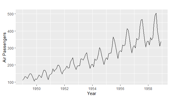
Figure 1. Training range data.Fifth, we do training range time series classical additive seasonal decomposition by moving averages with decompose function and store results within tsdec object. Within decompose function, parameters x = tdata includes training range data object, type = "additive" includes additive seasonal component and filter = NULL includes moving average with symmetric window. Notice that we have to evaluate whether time series classical additive or multiplicative seasonal decomposition is needed. Also, notice that decompose function parameters were only included as educational examples which can be modified according to your needs. Then we do time series decomposition chart with autoplot function. Within autoplot function, parameter object = tsdec includes training range time series decomposition.
In [5]:
tsdec <- decompose(x = tdata, type = "additive", filter = NULL)
autoplot(object = tsdec)
Out [5]: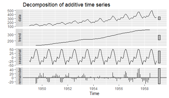
Figure 2. Training range time series classical additive seasonal decomposition by moving averages.References
[1] Data Description: Monthly international airline passenger numbers in thousands from 1949 to 1960.
Original Source: Box, G. E. P., Jenkins, G. M. and Reinsel, G. C. (1976). “Time Series Analysis, Forecasting and Control”. Third Edition. Holden-Day. Series G.
Source: datasets R Package AirPassengers Object. R Core Team (2021). “R: A language and environment for statistical computing”. R Foundation for Statistical Computing, Vienna, Austria.
[2] forecast R Package. Hyndman R, Athanasopoulos G, Bergmeir C, Caceres G, Chhay L, O’Hara-Wild M, Petropoulos F, Razbash S, Wang E, Yasmeen F (2022). “forecast: Forecasting functions for time series and linear models”. R package version 8.16
ggplot2 R Package. Hadley Wickham (2016). “ggplot2: Elegant Graphics for Data Analysis”. Springer-Verlag New York